Overview¶

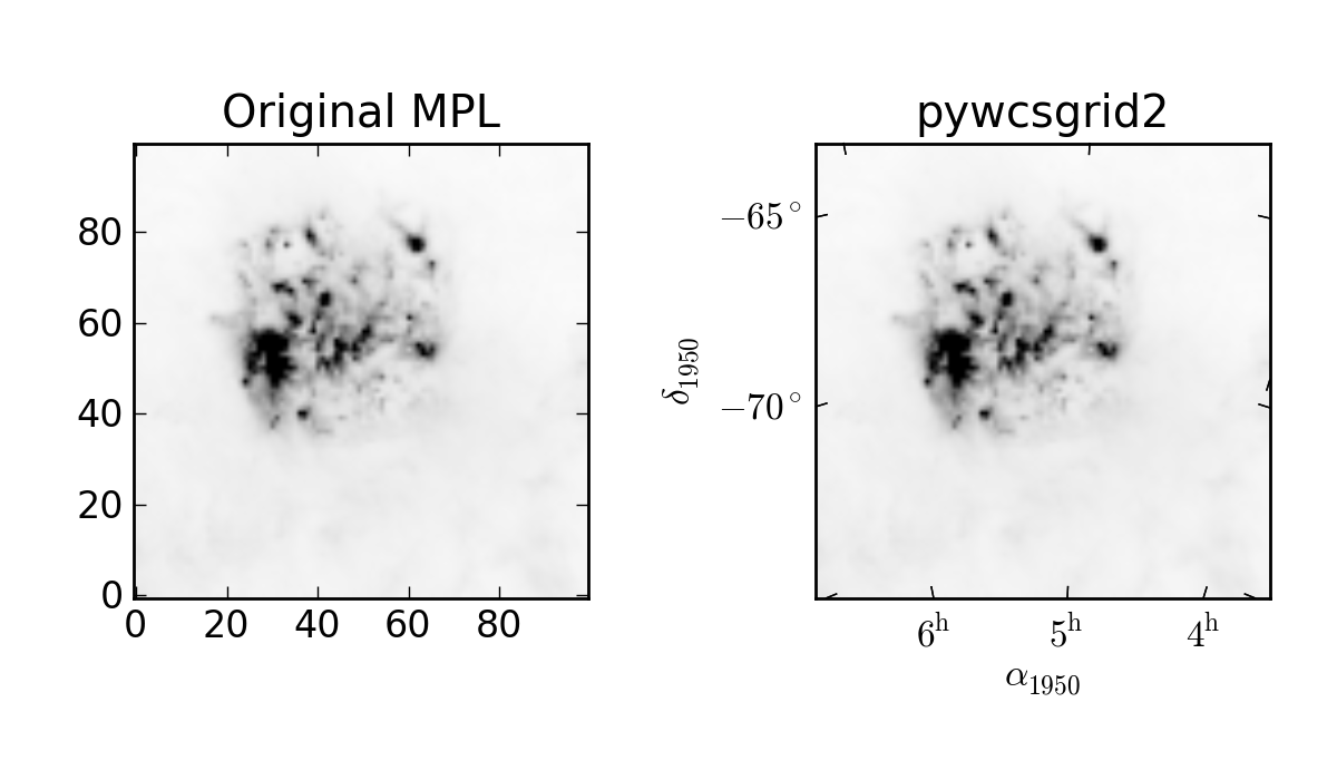
Basic Image Display¶

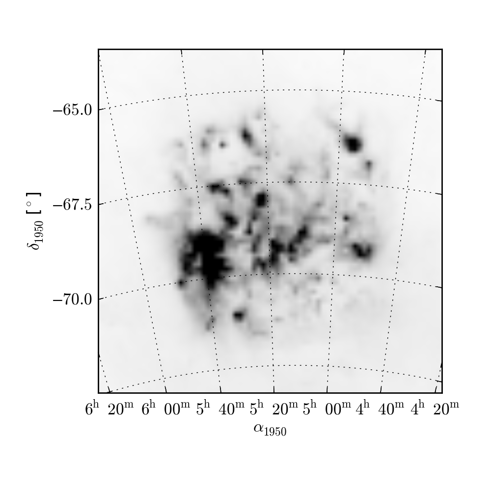
You read in the fits file using pyfits and create a subplot (or axes) using pywcsgrid2’s subplot command with its header (wcs) information.

import pyfits
import matplotlib.pyplot as plt

f = pyfits.open("data/lmc.fits")
h, d = f[0].header, f[0].data

# image display with mpl's original subplot(axes)
plt.subplot(121)
plt.imshow(d, origin="lower")


# image display with pywcsgrid2
import pywcsgrid2

pywcsgrid2.subplot(122, header=h)
plt.imshow(d, origin="lower")

[source code, hires.png, pdf]

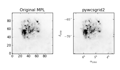
pywcsgrid2.subplot creates an instance of the pywcsgrid2.Axes class, which is derived from mpl’s Axes but draws ticks in proper sky coordinate. Note that the data coordinate of the AxesWcs axes is the image (pixel) coordinate ((0-based!) of the fits file. Only the ticklabels are displayed in the sky coordinates. For example, xlim and ylim needs to be in image coordinates (0-based).

ax = pywcsgrid2.axes([0.1, 0.1, 0.8, 0.8], header=h)

# viewlimits in image coordinate
ax.set_xlim(6, 81)
ax.set_ylim(23, 98)

As in the MPL, the grid method draws grid lines. It will draw curved grid lines using the given wcs information. Note that the ticks are also rotated accordingly.:

ax.grid()

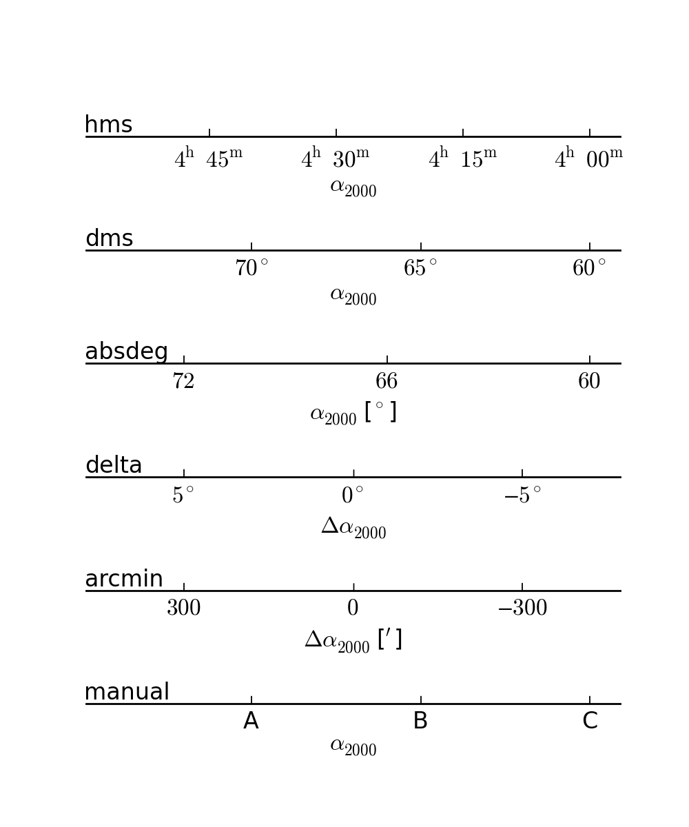
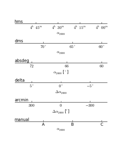
The axes in the pywcsgrid2 toolkit is based on mpl_toolkits.axisartist. Therefore, note that the mpl methods like set_ticks won’t work. For tick handling, pywcsgrid2 provides methods suitable for astronomical images. set_ticklabel_type changes the labeling of the ticks. For example,:

ax.set_ticklabel_type("hms", "dms")

make ticklabels in first axis (longitude) in the form of hour, minute and second and ticks in the second axis in the form of degree, minute and seconds. To change the ticklabeling of second axis into absoute degree:

ax.set_ticklabel_type("hms", "absdeg")

The ticklabel type of individual axis also can be changed.

ax.set_ticklabel2_type("absdeg", locs=[-65, -67.5, -70, -72.5])

Above example command makes the 2nd axis (dec.) of the absolute degree type with given tick locations.

Here are some examples of available ticklabel types.

[source code, hires.png, pdf]

See set_ticklabel1_type() for more details.

You may use locator_params command (which is introduced in mpl v1.0) to adjust the locator parameters.

ax.locator_params(axis="x", nbins=6)

[source code, hires.png, pdf]

Changing Cooditnate System¶

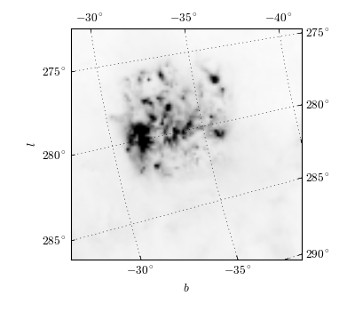
You can change the displayed sky coordinate (i.e., coordinates for ticks, ticklabels and grids). For example, to display the Galactic coordinate system:

ax.set_display_coord_system("gal")

The coordinate system must be one of “fk4”, “fk5”, or “gal”. Sometimes, you will need to swap the axis for better tick labeling (i.e., xaxis display latitude and yaxis display longitude).

ax.swap_tick_coord()

The pywcsgrid2.Axes class is derived from the mpl_toolkits.axisartist.axislines.Axes. For example, to turn on the top and right tick labels,:

ax.axis["top"].major_ticklabels.set_visible(True)
ax.axis["right"].major_ticklabels.set_visible(True)

[source code, hires.png, pdf]

Plotting in Sky Coordinate¶

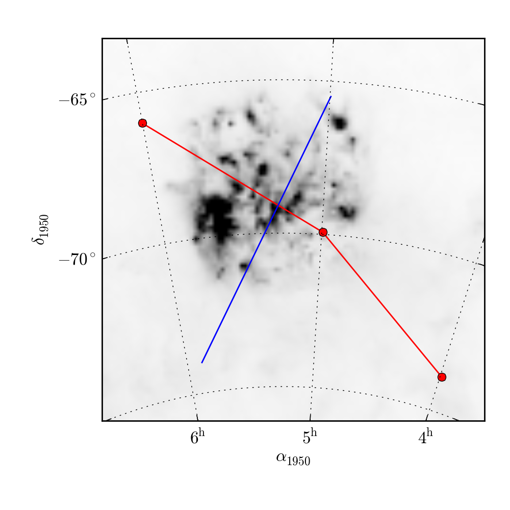
Again, the data coordinate of pywcsgrid2.Axes is a pixel coordinate (0-based) of the fits header (or any equivalent wcs information). For plot something in sky coordinate, you may convert your data into pixel coordinates, or you may use parasites axes (from mpl_toolkits.axes_grid) which does that conversion for you. For example, ax["fk5"] gives you an Axes whose data coordinate is in fk5 coordinate (available coordinates = “fk4”, “fk5”, “gal”). Most (if not all) of the valid mpl plot commands will work. The unit for the sky coordinates are degrees.:

# (alpha, delta) in degree
ax["fk4"].plot([x/24.*360 for x in [4, 5, 6]],
                [-74, -70, -66], "ro-")

# (l, b)  in degree
ax["gal"].plot([(285), (276.)],
               [(-30), (-36)])

[source code, hires.png, pdf]

Displaying Fits File of Different WCS¶

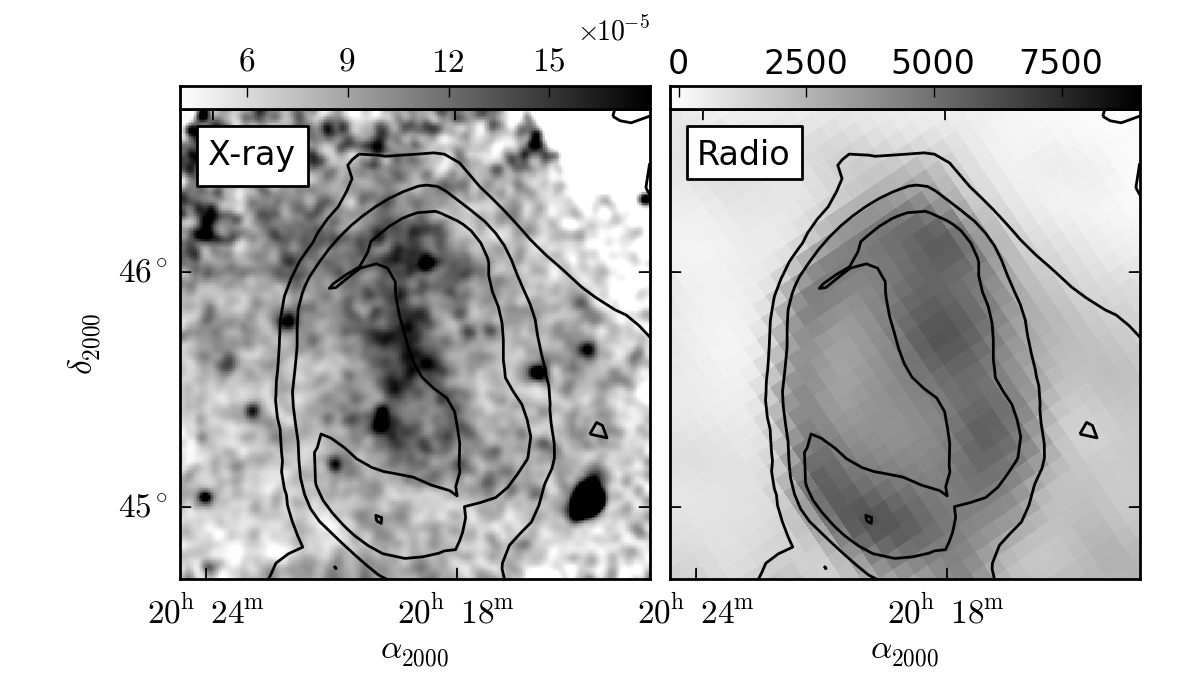
Often you need to compare two (or more) fits images with different WCS information. You may compare the image side by side. Or, you may show one of the image as contours an the other in pseudo-color (or gray) image. The AxesWcs supports parasite axes of different WCS header. For example, if ax is created with a header information h1, then ax[h2] have data coordinate of another header h2. Here is an example,

f1 = pyfits.open("f1.fits")
f2 = pyfits.open("f2.fits") # the WCS information is different from f1

h1, h2 = f1[0].header, f2[0].header

ax = pywcsgrid2.subplot(111, header=h1)
ax.imshow(f1[0].data) # working in pixel coordinate of h1

ax[h2].contour(f2[0].data) # in pixel coordinate of h2!

If you’re working on multiple axes, it is better to explicitly create GridHelper object and share them among multiple axes. Also, when you want to share both x and y-axis among axes and want to have equal aspect ratio, you may use adjustable=”box-forced” option.

grid_helper = pywcsgrid2.GridHelper(wcs=h1)

ax1 = pywcsgrid2.subplot(121, grid_helper=grid_helper,
                         aspect=1, adjustable="box-forced")
ax1.imshow(f1[0].data)

ax2 = pywcsgrid2.subplot(122, grid_helper=grid_helper,
                         aspect=1, adjustable="box-forced",
                         sharex=ax1, sharey=ax1)
ax2[h2].pcolormesh(f2[0].data)

When you use parasite axes (e.g., “ax[h2]”), most of plot commands (other than image-related routine) will work as expected. However, displaying images in other wcs coordinate system needs some consideration. You may simply use imshow

ax[h2].imshow(f2[0].data)

However, this will regrid the original image (f2[0].data) into the target wcs (regriding is necessary since matplotlib’s imshow only supports rectangular image). If you don’t want your data to be regridded, there are a few options available. You may use AxesWcs have imshow_affine method. With this, the image will be transformed by the backend (not by matplotlib) without regridding in matplotlib side.

ax[h2].imshow_affine(f2[0].data)

Since it uses an affine transform, it should not be used for images of large field of view where transformation is significantly non-linear. Also, this is only supported for agg backends and ps backend. Another option is to use a vector drawing command pcolormesh as in the above example. But pcolormesh is only optimized for agg backend and become extremely slow with increasing image size in other backends. Therefore, you may want to rasterize the pcolormesh (rasterization is fully supported in pdf and svg backend, and partially available in ps backend).

On the other hand, all the vector-oriented commands, such as contour, will work as expected.

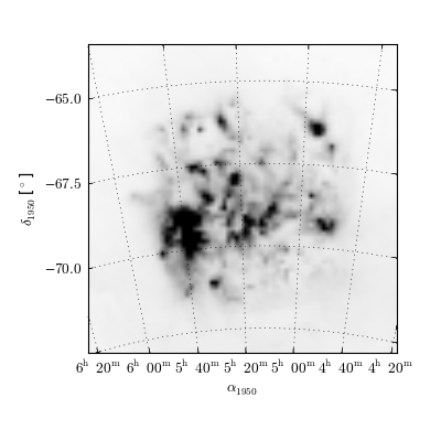
The example below is a more sophisticated one. The two fits images with different wcs are plotted using the mpl_toolkits.axes_grid1.AxesGrid. Both axes are created using the wcs information of the first image. Note that the gridhelper object is explicitly created and handed to the axes, i.e., the gridhelper is shared between two axes (this is to share tick label parameters). The second image, which has different wcs information is drawn using pcolormesh.

[source code, hires.png, pdf]

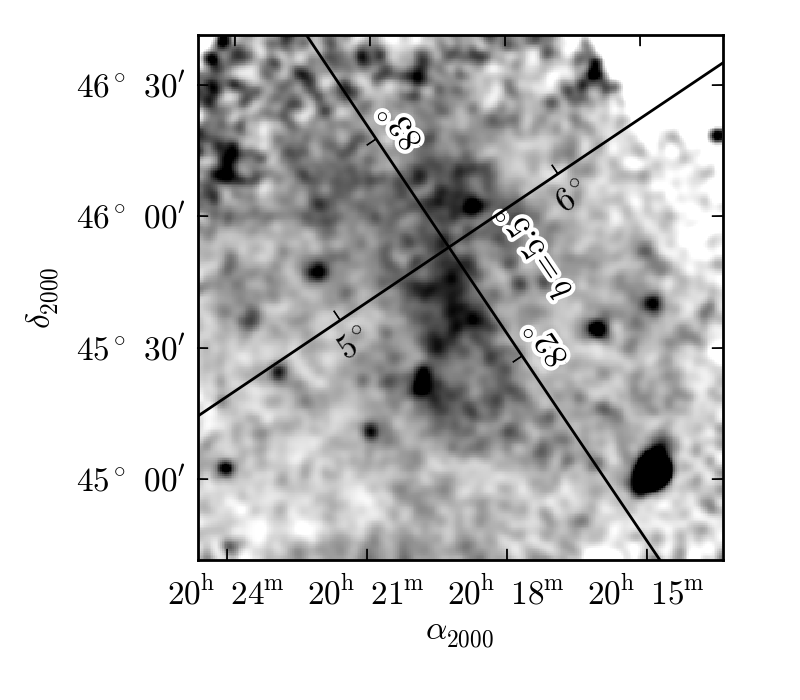
Floating Axis¶

It is possible to create a floating axis in any sky coordinate. This can be useful for drawing a Galactic object, where you draw a image in RA-Dec, but want to indicate the Galactic location of the object. A floating axis is created using the new_floating_axis method. The first argument indicate which coordinate, and the second argument is the value. For example, if you want to have a floating axis of b=0, i.e. the second coordinate (index starts at 0) is 0 in the Galactic coordinate:

axis = ax["gal"].new_floating_axis(1, 0.)
ax.axis["b=0"] = axis

See mpl_toolkits.axisartist for more about the floating axis.

Here is a complete example,

[source code, hires.png, pdf]

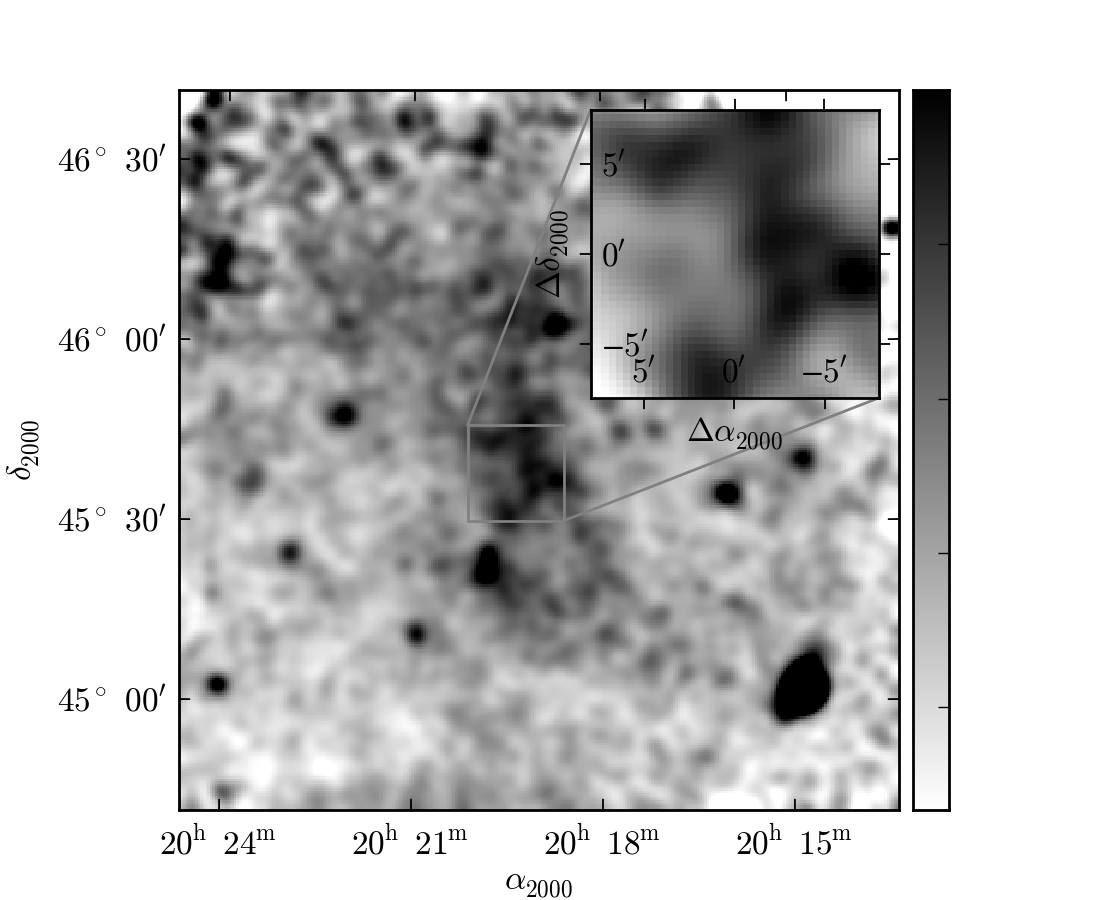
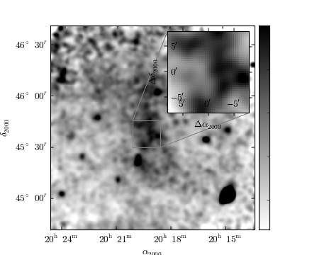
Inset Axes¶

pywcsgrid2 itself does not provide any particular functionality to support inset axes. However, inset axes is supported by the axes_grid1 toolkit, which can be seemingless utilized with pywcsgrid2. See axes_grid toolkit documentation for more details.

[source code, hires.png, pdf]

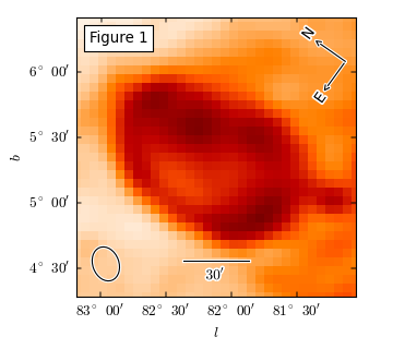
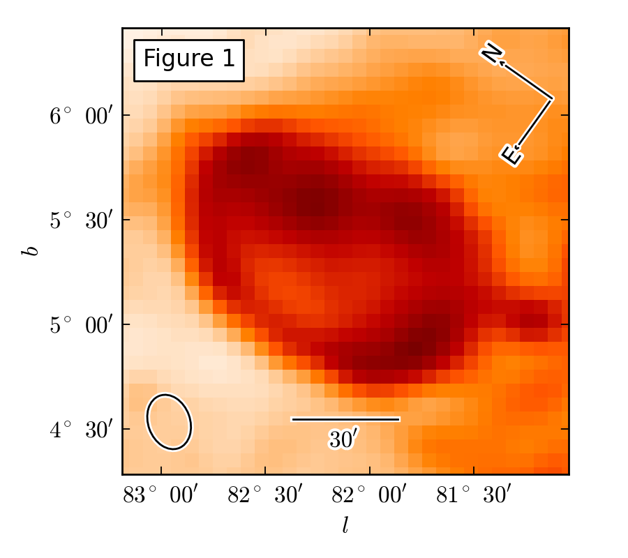
Axes Annotation¶

pywcsgrid2.Axes provides a few helper fucntion to annotate the axes. Most of them uses mpl_toolkits.axes_grid1.anchored_artists, i.e., the loc parameter in most of the commands is the location code as in the legend command.:

# Figure title
ax.add_inner_title("Figure 1", loc=2)

# compass
ax.add_compass(loc=1)

# Beam size
# (major, minor) = 3, 4 in pixel, angle=20
ax.add_beam_size(3, 4, 20, loc=3)

# Size
ax.add_size_bar(10, # 30' in in pixel
                r"$30^{\prime}$",
                loc=8)

[source code, hires.png, pdf]