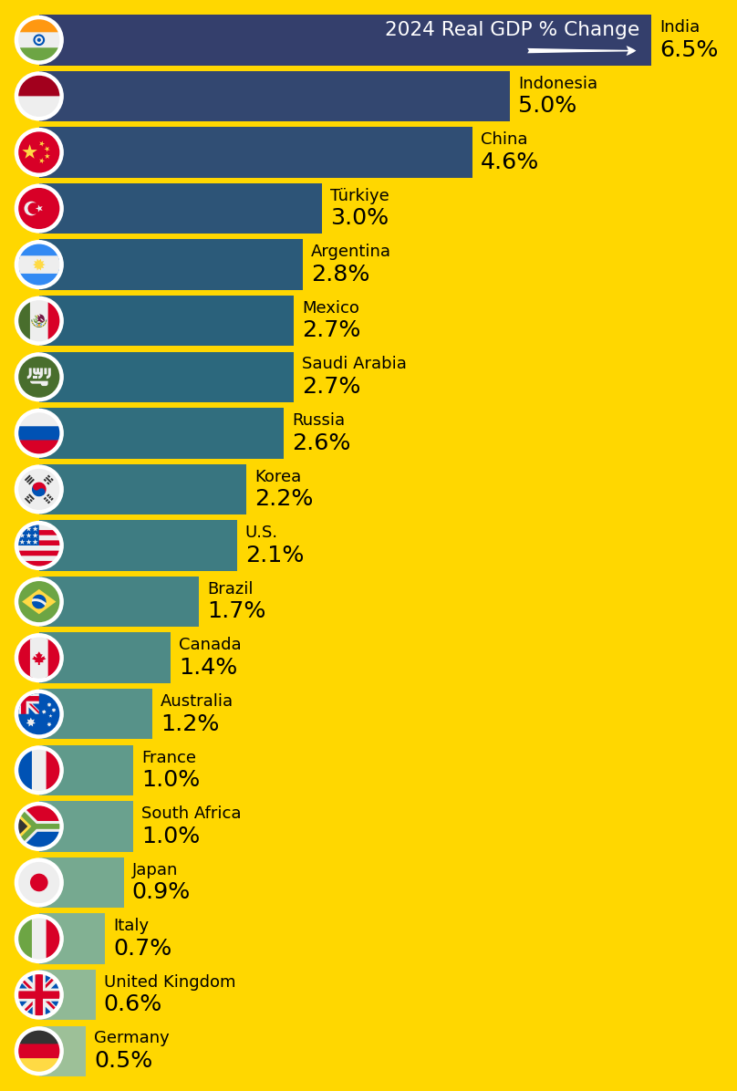
This post is to introduce mpl-flags package. To demonstrate the package, we would like to reproduce the plot from this post, only the barchart part.
Here is what the output will look like.
Code
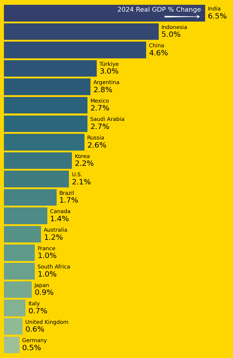
import matplotlib.pyplot as pltimport seaborn as snsfrom matplotlib.offsetbox import (TextArea, DrawingArea, AnnotationBbox, VPacker)from matplotlib.patches import Circlefrom mpl_flags import Flagsimport pandas as pdimport iocsvs ="""Country,2024 Real GDP % Change,CodeIndia,6.5,INIndonesia,5,IDChina,4.6,CNTürkiye,3,TRArgentina,2.8,ARMexico,2.7,MXSaudi Arabia,2.7,SARussia,2.6,RUKorea,2.2,KRU.S.,2.1,USBrazil,1.7,BRCanada,1.4,CAAustralia,1.2,AUFrance,1,FRSouth Africa,1,ZAJapan,0.9,JPItaly,0.7,ITUnited Kingdom,0.6,GBGermany,0.5,DE"""df = pd.read_csv(io.StringIO(csvs))fig, ax = plt.subplots(1, 1, num=1, figsize=(7, 10), clear=True, facecolor="gold")countries = df["Country"]gdp_changes = df["2024 Real GDP % Change"]country_codes = df["Code"]palette = sns.color_palette("crest", n_colors=len(countries))palette.reverse()sns.barplot(x=gdp_changes, y=countries, hue=countries, palette=palette, width=0.9, ax=ax)for country, gdp_change, bar inzip(countries, gdp_changes, ax.patches): t1 = TextArea(country, textprops=dict(size=10)) t2 = TextArea(f"{gdp_change}%", textprops=dict(size=14)) tt = VPacker(align="left", children=[t1, t2], sep=2) ab = AnnotationBbox(tt, (1, 0.5), xybox=(5, 0), frameon=False, xycoords=bar, boxcoords="offset points", box_alignment=(0., 0.5)) ax.add_artist(ab)flags = Flags("circle")kw =dict(frameon=False, box_alignment=(0.5, 0.5))for country, code, bar inzip(countries, country_codes, ax.patches):# draw white circular background around the flags da = DrawingArea(20, 20, clip=False) da.add_artist(Circle((10, 10), 15, ec="none", fc="w")) ab = AnnotationBbox(da, (0, 0.5), xycoords=bar, **kw) ax.add_artist(ab) da = flags.get_drawing_area(code, wmax=25) ab = AnnotationBbox(da, (0, 0.5), xycoords=bar, **kw) ax.add_artist(ab)from matplotlib.patches import FancyArrowPatchda = DrawingArea(70, 10, clip=False)arrow = FancyArrowPatch(posA=(0, 5), posB=(70, 5), arrowstyle='fancy,tail_width=0.2', connectionstyle='arc3', mutation_scale=15, ec="none", fc="w")da.add_artist(arrow) # Circle((10, 10), 15, ec="none", fc="w"))t1 = TextArea("2024 Real GDP % Change", textprops=dict(size=12, color="w"))tt = VPacker(align="right", children=[t1, da], sep=2)ab = AnnotationBbox(tt, (0.98, 0.5), xycoords=ax.patches[0], frameon=False, box_alignment=(1, 0.5))ax.add_artist(ab)fig.subplots_adjust(top=0.95, bottom=0.05)fig.set_facecolor("gold")ax.set_axis_off()plt.show()
mpl-flags
mpl-flags is a small packages to draw flags in your matplotlib plots It contains the flag data in vector format readily usable with Matplotlib. The original flags data are from svg format, converted to matplotlib’s Path data using mpl-simple-svg-parser. mpl-flags does not contain the original svg files, only the converted data in numpy format (vertices and codes).
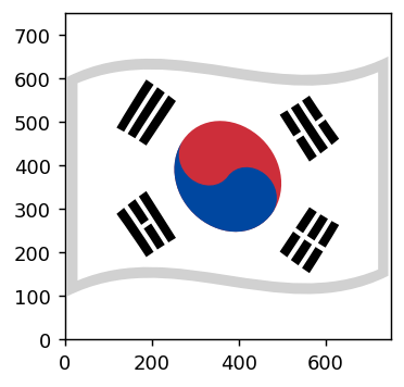
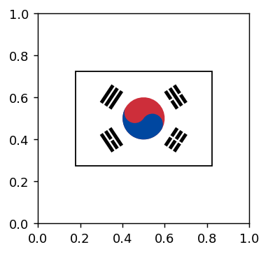
from mpl_flags import Flagsflags = Flags("noto_waved") # You initialize the Flags class specifying what kind of flags you like to use.# `noto_waved` is flags from google's noto emoji fonts.fig, ax = plt.subplots(figsize=(3, 3))flags.show_flag(ax, "KR")
show_flag method draws the flag in data coordinate.
The flag data is collected from various sources. Currently, it includes flags from
[All Codes]
AC AD AE AF AG AI AL AM AN AO AQ AR AS AT AU AW AX AZ BA BB BD BE BF BG BH
BI BJ BL BM BN BO BQ BR BS BT BV BW BY BZ CA CC CD CF CG CH CI CK CL CM CN
CO CP CQ CR CU CV CW CX CY CZ DE DG DJ DK DM DO DZ EA EC EE EG EH ER ES ET
EU FI FJ FK FM FO FR FX GA GB GD GE GF GG GH GI GL GM GN GP GQ GR GS GT GU
GW GY HK HM HN HR HT HU IC ID IE IL IM IN IO IQ IR IS IT JE JM JO JP KE KG
KH KI KM KN KP KR KW KY KZ LA LB LC LI LK LR LS LT LU LV LY MA MC MD ME MF
MG MH MK ML MM MN MO MP MQ MR MS MT MU MV MW MX MY MZ NA NC NE NF NG NI NL
NO NP NR NU NZ OM PA PC PE PF PG PH PK PL PM PN PR PS PT PW PY QA RE RO RS
RU RW SA SB SC SD SE SG SH SI SJ SK SL SM SN SO SR SS ST SU SV SX SY SZ TA
TC TD TF TG TH TJ TK TL TM TN TO TR TT TV TW TZ UA UG UK UM UN US UY UZ VA
VC VE VG VI VN VU WF WS XK XX YE YT YU ZA ZM ZW

[Missing Codes]
noto_original:  CQ AN PC SU XX UK YU FX
noto_waved:  CQ AN PC SU XX UK YU FX
1x1:  CQ AN AC SU UK YU FX EA TA
4x3:  CQ AN AC SU UK YU FX EA TA
circle:  PC
simple:  PC
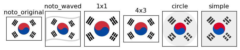
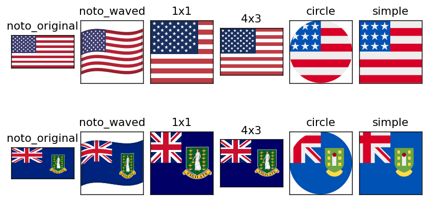
Above example of Korean flag is relatively simple and are modstly identical among kinds. However, for a bit complicated flags, different kinds show different flags. “circle” and “simple” show simplified flags without much details, best for small size, while other kinds reproduce the original flags.
mpl-flags package itself does not provide a mechanism to search for the country from common country name. For that, you may use packages like pycountry.
In the above example, we used show_flag method to draw the flag in data coordinate. Often, this is not you want. You want it to behave like texts.
Thus you are recommended to use get_drawing_area method. This returns matplotlib.offsetbox’s DrawingArea instance.
If you are not familar with these, you may take a look at this guide
<matplotlib.offsetbox.AnnotationBbox at 0x7fd5069febf0>
Now, let’s see how we can creat the barplots with flags. We will start the demo by loading the data as pandas DataFrame.
import pandas as pdimport iocsvs ="""Country,2024 Real GDP % Change,CodeIndia,6.5,INIndonesia,5,IDChina,4.6,CNTürkiye,3,TRArgentina,2.8,ARMexico,2.7,MXSaudi Arabia,2.7,SARussia,2.6,RUKorea,2.2,KRU.S.,2.1,USBrazil,1.7,BRCanada,1.4,CAAustralia,1.2,AUFrance,1,FRSouth Africa,1,ZAJapan,0.9,JPItaly,0.7,ITUnited Kingdom,0.6,GBGermany,0.5,DE"""df = pd.read_csv(io.StringIO(csvs))
Then, we will create a bar chart plot, without flags. Note that we are adding texts using AnnotationBbox and providing the bar itself as a coordinate, which means we will use a coordinate that is normalized to the extent of the bar.
# Set up the matplotlib figureimport matplotlib.pyplot as pltimport seaborn as snsfrom matplotlib.offsetbox import (TextArea, DrawingArea, AnnotationBbox, VPacker)from matplotlib.patches import FancyArrowPatchfig, ax = plt.subplots(1, 1, num=1, figsize=(7, 10), clear=True, facecolor="gold")countries = df["Country"]gdp_changes = df["2024 Real GDP % Change"]country_codes = df["Code"]palette = sns.color_palette("crest", n_colors=len(countries))palette.reverse()sns.barplot(x=gdp_changes, y=countries, hue=countries, palette=palette, width=0.9, ax=ax)# Add text labels of country name and percentagefor country, gdp_change, bar inzip(countries, gdp_changes, ax.patches): t1 = TextArea(country, textprops=dict(size=10)) t2 = TextArea(f"{gdp_change}%", textprops=dict(size=14)) tt = VPacker(align="left", children=[t1, t2], sep=2) ab = AnnotationBbox(tt, (1, 0.5), xybox=(5, 0), frameon=False, xycoords=bar, boxcoords="offset points", box_alignment=(0., 0.5)) ax.add_artist(ab)# For the top bar, we add text explaing the current plot.da = DrawingArea(70, 10, clip=False)arrow = FancyArrowPatch(posA=(0, 5), posB=(70, 5), arrowstyle='fancy,tail_width=0.2', connectionstyle='arc3', mutation_scale=15, ec="none", fc="w")da.add_artist(arrow) # Circle((10, 10), 15, ec="none", fc="w"))t1 = TextArea("2024 Real GDP % Change", textprops=dict(size=12, color="w"))tt = VPacker(align="right", children=[t1, da], sep=2)ab = AnnotationBbox(tt, (0.98, 0.5), xycoords=ax.patches[0], frameon=False, box_alignment=(1, 0.5))ax.add_artist(ab)# adjust subplot parameters and set the backgrond to gold.fig.subplots_adjust(top=0.95, bottom=0.05)fig.set_facecolor("gold")ax.set_axis_off()
We are now going to add flags. If you know how annoatation_box works, adding flags is very straight forward. In the example below, we will create two DrawingArea per bar. The first one is to draw a white background circle for the flags. And another DrawingArea for flags of circle kind.
from matplotlib.patches import Circlefrom mpl_flags import Flagsflags = Flags("circle")kw =dict(frameon=False, box_alignment=(0.5, 0.5))for country, code, bar inzip(countries, country_codes, ax.patches):# draw white circular background around the flags da = DrawingArea(20, 20, clip=False) # since we are using box_aligment=(0.5, 0.5) and clip=Flase,# the size of Drawing Area does not realy matter da.add_artist(Circle((10, 10), 15, ec="none", fc="w")) # place the circle at the center of the drawing_area. ab = AnnotationBbox(da, (0, 0.5), xycoords=bar, **kw) ax.add_artist(ab)# Now we draw flags. da = flags.get_drawing_area(code, wmax=25) ab = AnnotationBbox(da, (0, 0.5), xycoords=bar, **kw) ax.add_artist(ab)
no gradient support
Some flags (the original svg files) use gradient, which is not currently supported by mpl-flags. Below, we compare original svg file (left) and mpl-flags flag rendering. You will notice what mpl-flags result misses some colors.
# list of flags with gradientwith_gradients = {"noto_original": ['BZ', 'EC', 'FK', 'GS', 'GT', 'MX', 'NI', 'PM', 'TA', 'VG'],"4x3": ['BZ', 'FK', 'GS', 'GT', 'MX', 'NI', 'VG']}