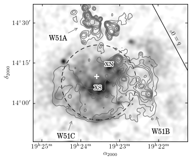
W51C X-ray and Radio

Data preparation

import pyfits
import scipy.ndimage as ni

f_X = pyfits.open("w51c/xselrosat_image.xsl")
d_X = ni.gaussian_filter(f_X[0].data.astype("d"), 5)
h_X = f_X[0].header

f_R = pyfits.open("w51c/w51_vgps.fits")
d_R, h_R = f_R[0].data, f_R[0].header

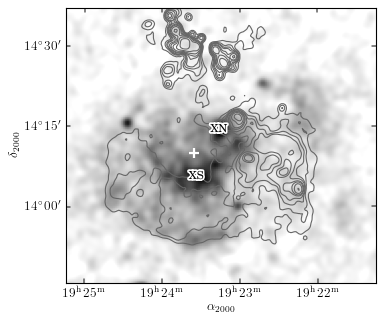
We create an axes using pywcsgrid2. We use header information of the X-ray image.

import pywcsgrid2
plt.figure(1, figsize=(5,5))
ax = pywcsgrid2.subplot(111, header=h_X)

Note that the data coordinate of the pywcsgrid2’s Axes is pixel coordinate of the given header. Thus we can show the image as.

im = ax.imshow(d_X, origin="lower", cmap=plt.cm.gray_r)
im.set_clim(0.11, 0.7)

We now adjust the x- and y-lim. Remember, these are in pixel coordinate. And turn off auto adjustment of x- and y-lim.

ax.set_xlim(363, 827)
ax.set_ylim(349, 761)
ax.set_autoscale_on(False)

We mark a position with plot command. While the data coordinate of the axes is the pixel coordinate of the fits file, a parasite axes whose data coordinate is “fk5” can be created by indexing the axes with “fk5”, e.g., ax[“fk5”]. Similarly, ax[“fk4”] and ax[“gal”] are also available. Below, we use ax[“fk5”].plot command whose coordinate is interpreted as world coordinate in fk5 (in degree).

ax["fk5"].plot([290.896], [14.1669], "w+", ms=9, mew=2, zorder=3)

We put some annotations. We again use a parasite axes. Note also that we use patheffects.

# annotate XN and XS
from matplotlib.patheffects import withStroke
myeffect = withStroke(foreground="w", linewidth=3)
kwargs = dict(path_effects=[myeffect])

t1 = ax["fk5"].annotate("XN", (290.817, 14.245), size=10,
                 ha="center", va="center",
                 **kwargs)
t2 = ax["fk5"].annotate("XS", (290.890, 14.099), size=10,
                 ha="center", va="center",
                 **kwargs)

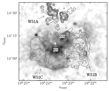
Now we draw contour lines of radio images. The radio fits has different wcs information than the X-ray one. We use pywcsgrid2’s parasite axes feature. If we index a pywcsgrid2’s axes with a pyfits header, it creates an parasite axes whose data coordinate is that of the pixel coordinate of the given header. In the example below, we index as “ax[h_R]”. This returns an axes whose data coordinate is that of the radio file(h_R).

cont = ax[h_R].contour(d_R,
                      [40, 60, 80, 100, 150, 200,
                       300, 500, 1000], colors="w")
[cl.set_color("0.4") for cl in cont.collections] # to change contour colors

Put more annotations with arrow.

# Mark W51C, W51A, W51B
kwargs = dict(arrowprops=dict(arrowstyle="->", ec=".5",
                              relpos=(0.5, 0.5)),
              bbox=dict(boxstyle="round", ec="none", fc="w"))

ann1 = ax.annotate("W51C", xy=(481, 415),
                   xytext=(-10, -25), textcoords="offset points",
                   ha="center", va="top", **kwargs)

ann1 = ax.annotate("W51B", xy=(732, 428),
                   xytext=(10, -25), textcoords="offset points",
                   ha="center", va="top", **kwargs)

ann1 = ax.annotate("W51A", xy=(501, 691),
                   xytext=(-20, -15), textcoords="offset points",
                   ha="right", va="top", **kwargs)

Using pyregion module, you can draw ds9 region files.

# draw XMM Mos region
import pyregion
reg = pyregion.open("w51c/mos_fov.reg").as_imagecoord(h_X)
patches, txts = reg.get_mpl_patches_texts()
circ = patches[0]
ax.add_patch(circ)

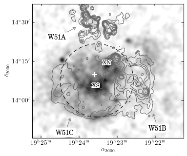
where the contents of “mos_fov.reg” is

fk5; circle(290.88372,14.130298,843.31194") # color=black dash=1

As a last step, we show a line of “b=0”. We use floating axis feature.

ax.axis["b=0"] = ax["gal"].new_floating_axis(1, 0.)

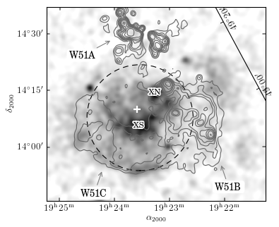
This creates a floating axis in galactic coordinates whose second coordinate (first argument 1. Index starts from 0) has a value of 0. We disable ticks and ticklabels and set axis label.

ax.axis["b=0"].toggle(all=False, label=True)
ax.axis["b=0"].label.set_text(r"$b=0^{\circ}$")