LMC

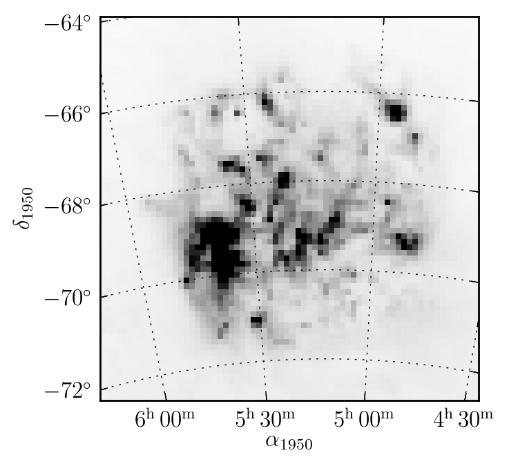
One of the strength of pywcsgrid2 is its ability to handle curved coordinate system. This is especially useful for images of large field of view (or all-sky maps) where the sky curvature is significant. Here we demosntrate this with the IRAS image of Large Magellanic Cloud.

Data preparation

import pyfits
f = pyfits.open("tutorial/lmc.fits")
d, h = f[0].data, f[0].header

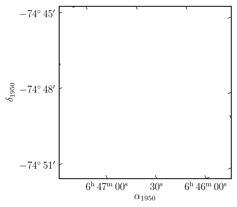
We create a subplot using pywcsgrid2 with the header information.

import pywcsgrid2

plt.figure(1, [4,3.5])

ax = pywcsgrid2.subplot(111, header=h) # this is pywcsgrid2 version of
                                       # mpl's subplot command.

plt.tight_layout()
plt.show()

[hires.png, pdf]

pywcsgrid2.subplot is analgous to mpl’s subplot command. In addtion to usual mpl’s subplot parameters (it internally calls mpls’s subplot command so all its argument will work), a user shoud specify the wcs information; here we provide header object (pyfits must be used). Note that the data coordinate of the pywcsgrid2’s Axes is pixel coordinate of the given header. The coordinate is 0-based, i.e., center of the bottom-left corner pixel has the coordinate of (0, 0). Note that newly created axes by default have x, y limits of (0, 1), which is the default behavior of matplolib.

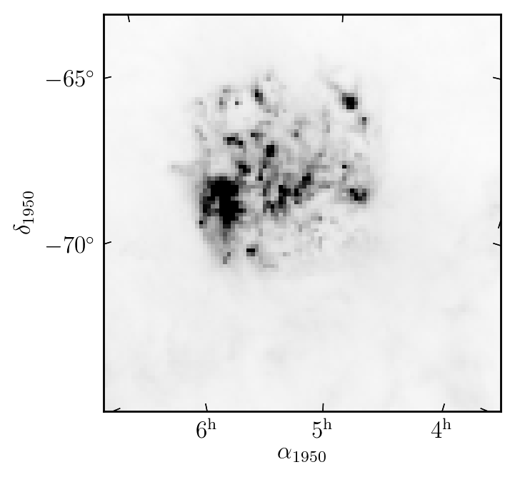
To show the image data, you just call imshow, as you do with matpltolib. Since the data coordinate is pixel coordinate of the given image, simple imshow is sufficient here.

ax.imshow(d, origin="low", vmin=0, vmax=2000,
          cmap=plt.cm.gray_r)

[hires.png, pdf]

(Note that you need to call plt.draw() or plt.show() to see changed figure).

Note that some ticks are rotated (this is more clear in the high res. figure). In pywcsgrid2, ticks are directed along the coordinate lines (i.e., grid lines). This can be seen more clearly if we draw grid lines.

ax.grid()

[hires.png, pdf]

To change the viewing limits of axes, simply call set_xlim or set_ylim remembering that the values should be given in pixel coordinate. Of course you can use zoom and pan button in the toolbar.

ax.set_xlim(8.5, 76.5)
ax.set_ylim(25.5, 94.5)

[hires.png, pdf]

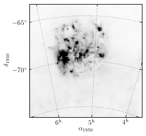
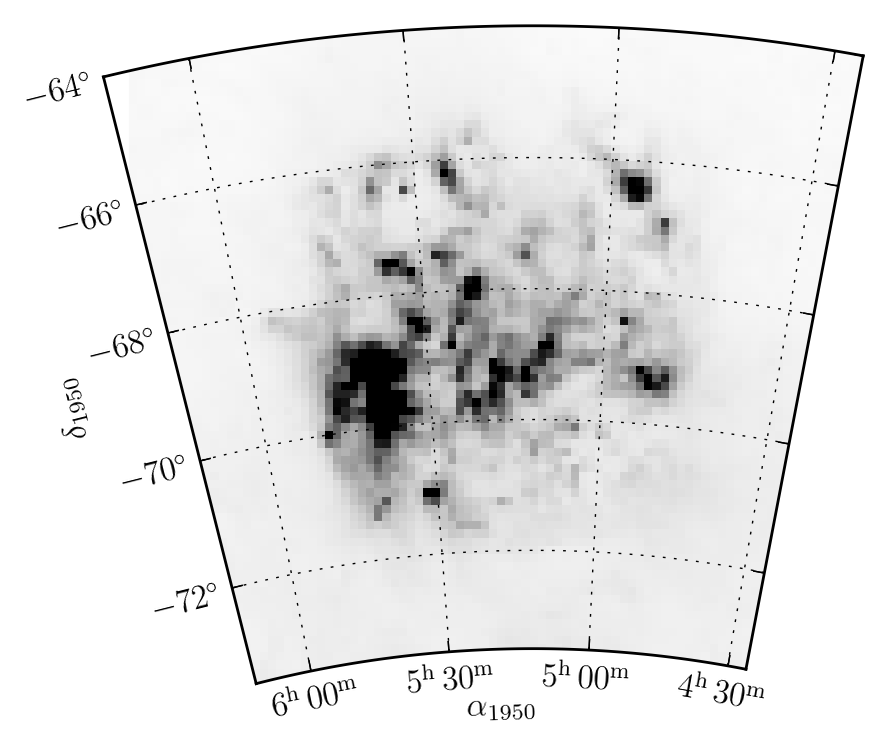
pywcsgrid2 has some support for floating axes. You must specify the limits of longitude and latitude.

import pyfits, pywcsgrid2

plt.figure(figsize=[5, 5])

f = pyfits.open("tutorial/lmc.fits")

extremes=93.0, 66.5, -73.5, -64
# ra : 93.0 ~ 66.5 (in degree, the order matters)
# dec : -73.5 ~ -64

ax = pywcsgrid2.floating_subplot(111, header=f[0].header,
                                 extremes=extremes)

ax.imshow(f[0].data, origin="low", vmin=0, vmax=2000,
          cmap=plt.cm.gray_r)

ax.grid()

[hires.png, pdf]